Architecture & Data Flow#
This section provides a simplified explanation of Leaspy’s internal architecture from a code perspective. Even if this guide could seem long and tedious, we simplified the work for over 200 files and dousents of functions in just some modules. You have two ways to read it: taking a look to the simplified versions here, or take a look to the modules you want to have a deeper inderstanding about how works leaspy inside. If you are not going to developpe new features/methods, the overview is enough.
Key steps include:
Data Preparation: Adapting raw data and putting it into the
Dataformat.Model Fitting: Creating a model (e.g.
model = LogisticModel(...)) and fitting it (model.fit(...)).Personalization (Optional): Estimating individual trajectories for each patient (
model.personalize(...)).
This guide offers two levels of depth: a global explanation and a detailed deep-dive. Feel free to explore according to your needs.
High-Level Overview#
When you run a method, a lot happens under the hood. Here is a simplified code snippet that runs a LogisticModel:
from leaspy.io.data import Data
from leaspy.models import LogisticModel

data = Data.from_dataframe(alzheimer_df)		# Data part
model = LogisticModel(name="test-model",
	source_dimension=2)			# Model creation
model.fit(data, "mcmc_saem", seed=42,
    n_iter=100,progress_bar=False)		# Fitting
Inside the leaspy library, most of the code you interact with is organized into modules, which contain classes. A class bundles methods (functions attached to the class) and attributes (data stored on the object). For example, the LogisticModel.py module defines two classes, each providing its own methods and attributes.
You can visualize the structure of the logistic (inside /src/leaspy/models/logistic.py) module like this:
        %%{init: {"flowchart": {"rankSpacing": 10, "nodeSpacing": 20}} }%%
flowchart TD
    %% Softer cohesive palette (indigo/lilac/teal/sand)
    classDef module fill:#EEF2FF,stroke:#4F46E5,stroke-width:2px,color:#1F2A5A,rx:8,ry:8;
    classDef cls    fill:#F3E8FF,stroke:#7C3AED,stroke-width:2px,color:#3B0764,rx:8,ry:8;
    classDef method fill:#E6FFFB,stroke:#0F766E,stroke-width:1px,color:#134E4A,rx:6,ry:6;
    classDef attr   fill:#FFF7ED,stroke:#C2410C,stroke-width:1px,color:#7C2D12,rx:6,ry:6;

    %% Micro spacer (nearly zero height)
    classDef micro fill:transparent,stroke:transparent,color:transparent,font-size:1px;

    %% Module Subgraph
    subgraph Module["__Module: logistic(.py)__"]
        direction TB

        %% tiny spacer so the subgraph title doesn't get overlapped
        ModuleMicro["."]:::micro

        %% Class 1: Mixin (no pad inside -> less empty space)
        subgraph ClassMixin["__Class: LogisticInitializationMixin__"]
            direction TB
            Method1("Method: _compute_initial_values_for_model_parameters"):::method
        end

        %% Class 2: Model
        subgraph ClassModel["__Class: LogisticModel__"]
            direction TB
            Attr1("Attribute: name"):::attr
            Method2("Method: \__init__"):::method
            Method3("Method: get_variables_specs"):::method
            Method4("Method: metric"):::method
            Method5("Method: model_with_sources"):::method

            %% Force vertical listing inside the class
            Attr1 --> Method2 --> Method3 --> Method4 --> Method5
        end

        %% Force vertical stacking of the two class subgraphs
        ClassMixin --> ClassModel

        %% Anchor the micro node so it actually affects layout
        ModuleMicro --> ClassMixin
    end

    %% Apply Classes
    Module:::module
    ClassMixin:::cls
    ClassModel:::cls

    %% Hide all layout-forcing edges (keeps it clean)
    linkStyle default stroke:transparent,stroke-width:0;
This example allows us to see how is structured a module, we will go deeper in the other modules that compose the worflow from leaspy, specially in the most the most simple scenario: a logistic regression.
Simplified workflow structure#
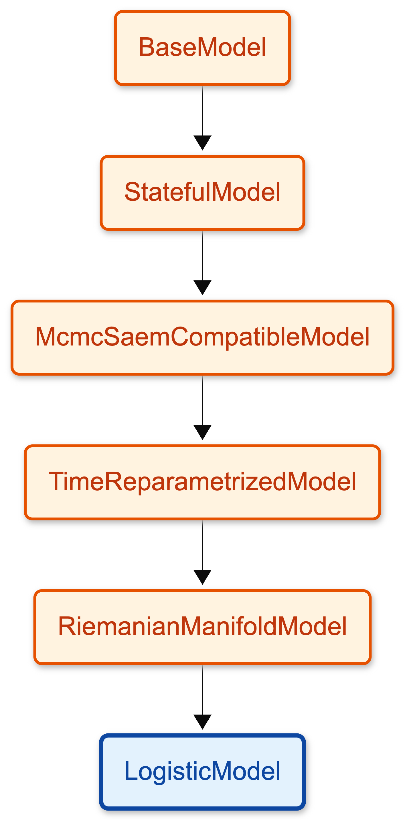
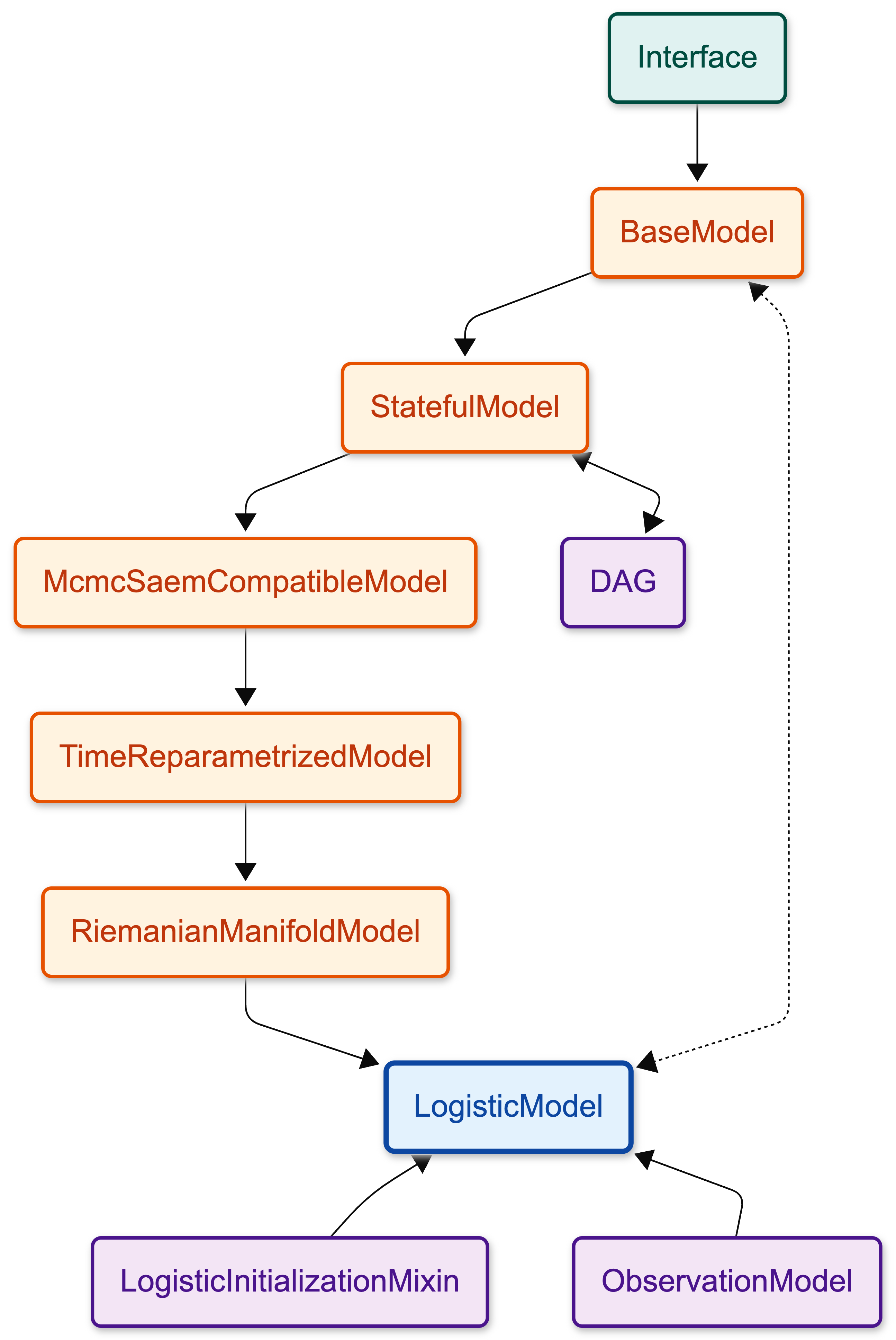
When you create your model and you fit it a lot happens under the hood. For instance LogisticModel inherits methods and attributes from other classes in a chain. LogisticModel inherits from RiemanianManifoldModel, which inherits from other classes, and so on.
Here is the inheritance chain for the Logistic model. You can click on the nodes to see the details of each class. The diagram in the “Simplified version” tab highlights the essential modules for a standard logistic regression execution, offering a cleaner starting point. The “Complete version” shows the full inheritance hierarchy.
Why This Architecture?#
While you could theoretically write a LogisticModel as one massive 5000-line class, Leaspy breaks it down into a compositional inheritance chain. Each class in the diagram above adds a specific layer of capability:
Reusability:
LinearModelandJointModelreuse 90% of the same code asLogisticModel(parameter storage, algorithm compatibility). They only override the final mathematical formulas.Extensibility: If you want to create a model with a different time behavior, you don’t start from scratch. You might branch off after
McmcSaemCompatibleModeland implement your own time reparameterization, while keeping all the algorithm compatibility for free.
This “layer” approach means complex features (like Riemannian manifold geometry or MCMC sampling) are implemented once and shared across all models, rather than being copy-pasted into every new model type.
You can read the Simplified Overview below for a quick summary of how all these pieces fit together, or follow the path in the table of contents to explore each module in depth one by one.
Simplified Overview
To perform a logistic regression, Leaspy coordinates a stack of specialized modules that transform raw data into a mathematical trajectory.
The Mathematical Core It begins with the Observation Model, which links your noisy measurements to the theoretical curves. Underlying this is the Logistic Model, which imposes the specific S-shape of the progression, supported by the Riemannian Manifold Model which handles the geometric mixing of multiple biomarkers. The Time Reparametrized Model personalizes this process by warping the timeline for each subject.
The Software Infrastructure
Supporting this math is a robust backend. ModelInterface and BaseModel define the standard blueprint and orchestration logic (like .fit()). StatefulModel acts as the model’s memory, holding the actual values of parameters during execution. Finally, McmcSaemCompatibleModel acts as a translator, ensuring the model provides the specific statistics needed by the generic MCMC-SAEM optimization algorithm.
If you want more details about a specific module, you can click on its corresponding node in the index. For now, let’s start with the base of the inheritance chain: ModelInterface.