The Variables DAG#

Module: leaspy.variables.dag

document: leaspy.variables.dag.VariablesDAG

Why does Leaspy need a DAG?#

A Leaspy model is not a simple function \(f(x; \theta)\). It has many variables of different natures (data, parameters, latent variables, derived quantities), and they form a dependency chain: some variables can only be computed once others are known.

For example, in the logistic model:

You cannot compute the reparametrized time rt until you know the patient’s time-shift tau and acceleration alpha.
You cannot compute alpha until you sample the latent variable xi.
You cannot compute the model output until you have rt, the metric, and the population parameter g.

The VariablesDAG is the data structure that encodes all of these relationships. It answers two critical questions at runtime:

Forward propagation: “Given that I just assigned a value to variable X, which downstream variables need to be (re)computed?”
Classification: “Which variables are parameters? Which are individual latent variables? Which are derived?”

Without it, every algorithm would need model-specific hard-coded logic. With it, the MCMC-SAEM algorithm can remain generic: it proposes a new value for a latent variable, and the DAG ensures consistency propagates automatically.

What is a DAG, concretely?#

A Directed Acyclic Graph is a set of nodes (variables) connected by directed edges (dependencies), with no cycles.

Directed: each edge has a direction: “A is needed to compute B” (A → B).
Acyclic: there is no circular chain like A → B → C → A.

In code, VariablesDAG is a frozen dataclass that stores:

Attribute	What it holds
`variables`	A mapping from variable name → variable specification object
`direct_ancestors`	For each variable, the set of variables it directly depends on
`direct_children`	(precomputed) For each variable, the set of variables that depend on it
`sorted_variables_names`	All variable names in topological order (roots first, leaves last)
`sorted_children`	For each variable, all downstream descendants (transitive closure)
`sorted_ancestors`	For each variable, all upstream ancestors (transitive closure)
`sorted_variables_by_type`	Variables grouped by their Python type (`ModelParameter`, `IndividualLatentVariable`, etc.)

The topological sort guarantees that when computing values top-to-bottom, every variable’s inputs are already available.

The Logistic Model’s DAG#

Below is the complete dependency graph for a multivariate LogisticModel with sources. Each node is a variable in the model; each arrow means “this variable is needed to compute that one”. The graph is organized into three conceptual sections — Temporal Variability, Geometrical Model, and Spatial Variability — that merge at the top into the observation model and the negative log-likelihood.

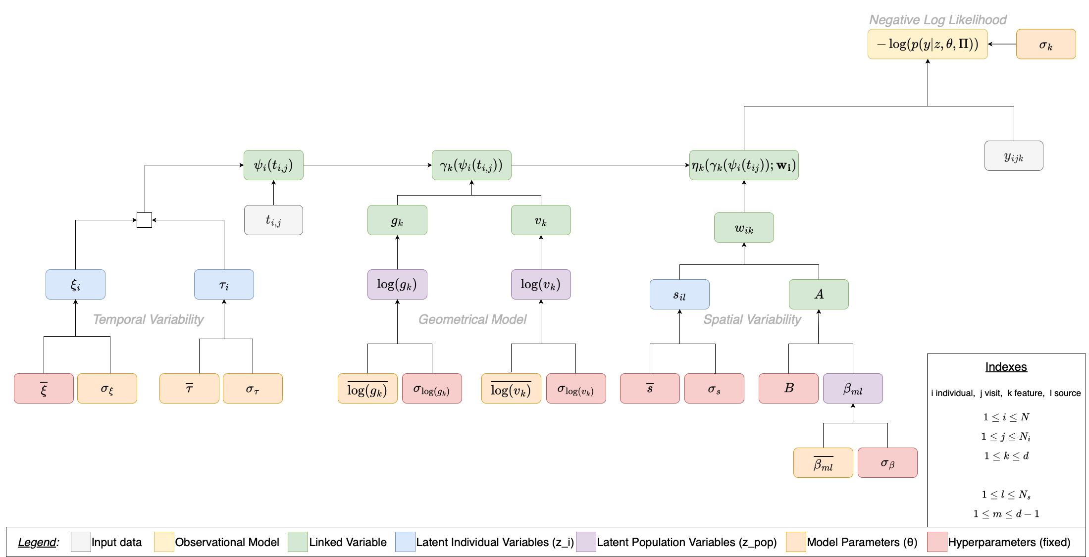
Legend (variable types):

Input data — observed values provided by the dataset
Observational Model — likelihood computation
Linked / Derived — deterministically computed from parents
Individual latent variables \(z_i\) — sampled per patient (E-step)
Population latent variables \(z_{pop}\) — sampled at population level (E-step)
Model parameters \(\theta\) — estimated during optimization (M-step)
Hyperparameters — fixed priors, not learned

Section-by-section breakdown#

Each tab below isolates one section of the diagram, shows its sub-graph, and explains every variable.

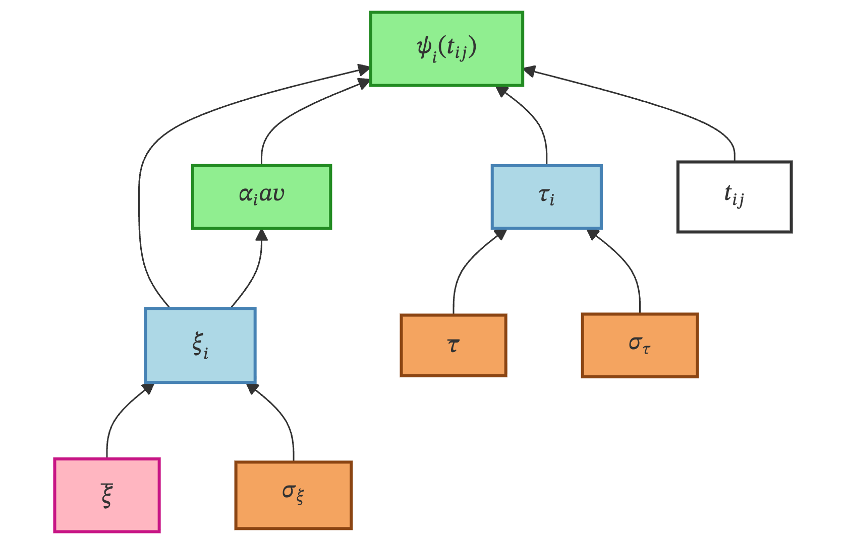
Temporal Variability governs when each patient’s disease trajectory is positioned on the time axis. It introduces two individual latent variables — a time-shift \(\tau_i\) and an acceleration factor \(\xi_i\) — that together define a patient-specific time reparametrization.

Variables#
Variable & Type	Description
\(\overline{\xi}\) — Hyperparameter	Mean of the acceleration factor distribution. Fixed at 0.0, so the prior mode of \(\alpha_i = \exp(\xi_i)\) is 1 (meaning “average speed”). Code name: `xi_mean`. Origin/Definition: `RiemanianManifoldModel.get_variables_specs()`
\(\sigma_\xi\) — Model parameter	Standard deviation of \(\xi_i\). Estimated during the M-step — controls how much acceleration varies across patients. Code name: `xi_std`. Origin/Definition: `TimeReparametrizedModel.get_variables_specs()`
\(\xi_i\) — Individual latent	Acceleration factor (log-scale) for patient \(i\). Sampled from \(\mathcal{N}(\overline{\xi},\; \sigma_\xi^2)\). Code name: `xi`. Origin/Definition: `TimeReparametrizedModel.get_variables_specs()`
\(\alpha_i\) — Linked	Individual acceleration: \(\alpha_i = \exp(\xi_i)\). Deterministic transform. Code name: `alpha`. Origin/Definition: `TimeReparametrizedModel.get_variables_specs()`
\(\overline{\tau}\) — Model parameter	Population mean of the time-shift. Estimated — represents the “average age of onset”. Code name: `tau_mean`. Origin/Definition: `TimeReparametrizedModel.get_variables_specs()`
\(\sigma_\tau\) — Model parameter	Standard deviation of \(\tau_i\). Estimated — controls how spread out disease onset ages are. Code name: `tau_std`. Origin/Definition: `TimeReparametrizedModel.get_variables_specs()`
\(\tau_i\) — Individual latent	Time-shift for patient \(i\). Sampled from \(\mathcal{N}(\overline{\tau},\; \sigma_\tau^2)\). Code name: `tau`. Origin/Definition: `TimeReparametrizedModel.get_variables_specs()`
\(t_{ij}\) — Input data	Observed timepoints (visit ages). Code name: `t`. Origin/Definition: `McmcSaemCompatibleModel.get_variables_specs()`
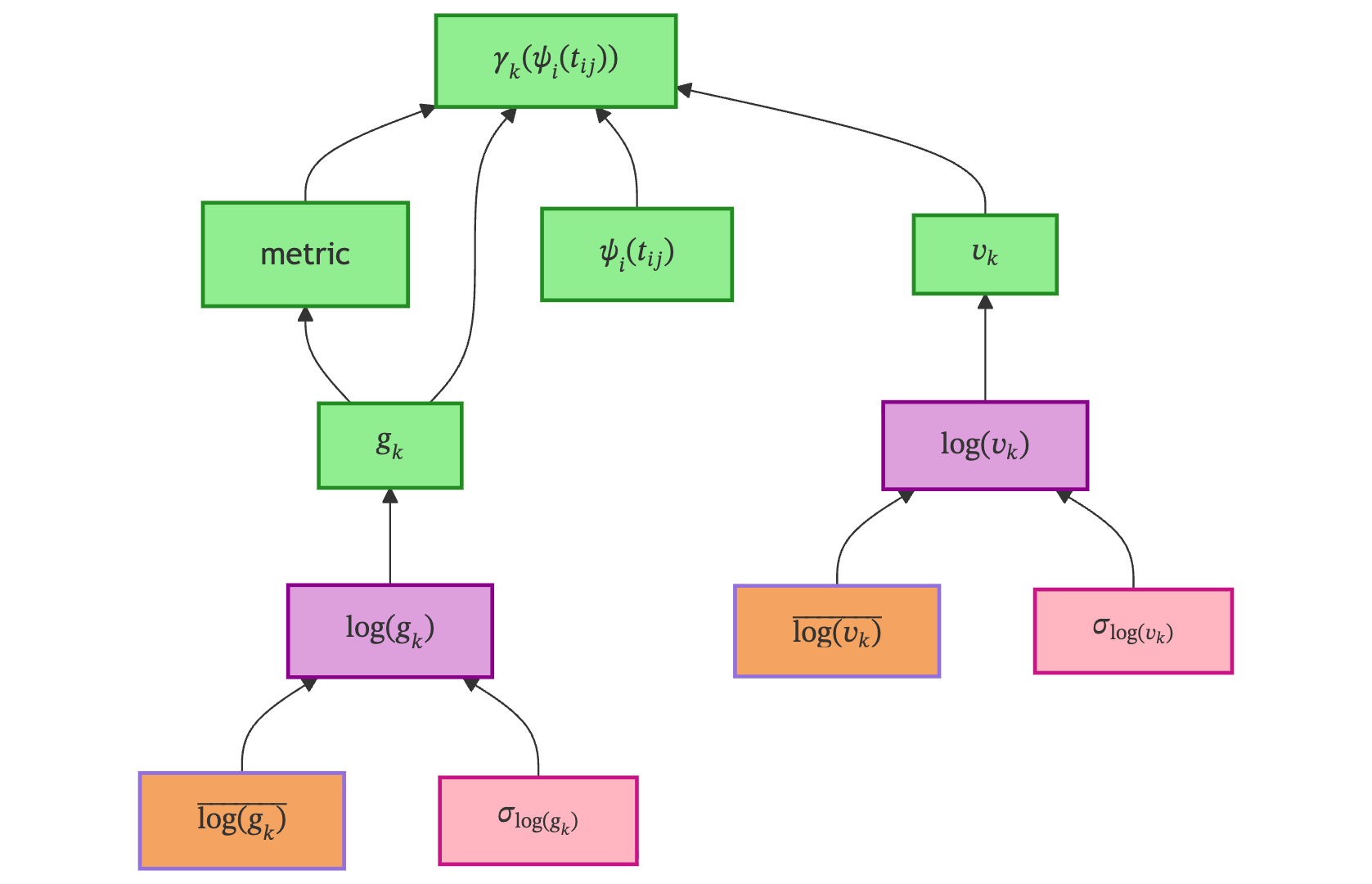
\(\psi_i(t_{ij})\) — Linked	Reparametrized time: \(\psi_i(t_{ij}) = \alpha_i \cdot (t_{ij} - \tau_i)\). This is the patient-specific “disease clock”. Code name: `rt`. Origin: `TimeReparametrizedModel.get_variables_specs()`. Definition: `TimeReparametrizedModel.time_reparametrization`

Geometrical Model defines the shape of the disease trajectory on the Riemannian manifold. It introduces population-level parameters \(g_k\) (position) and \(v_k\) (velocity) for each feature \(k\), and combines them with the reparametrized time to produce the per-feature trajectory \(\gamma_k\).

Variables#
Variable & Type	Description
\(\overline{\log(g_k)}\) — Model parameter	Mean of the log-position prior. Estimated — determines where each feature’s sigmoid is centered (midpoint value). Code name: `log_g_mean`. Origin/Definition: `LogisticModel.get_variables_specs()`
\(\sigma_{\log(g_k)}\) — Hyperparameter	Standard deviation of \(\log(g_k)\). Fixed at 0.01 to keep \(g_k\) close to its mean. Code name: `log_g_std`. Origin/Definition: `LogisticModel.get_variables_specs()`
\(\log(g_k)\) — Population latent	Log-position for feature \(k\). Sampled from \(\mathcal{N}(\overline{\log(g_k)},\; \sigma_{\log(g_k)}^2)\). Code name: `log_g`. Origin/Definition: `LogisticModel.get_variables_specs()`
\(g_k\) — Linked	Position parameter: \(g_k = \exp(\log(g_k))\). Controls the midpoint of the sigmoid for feature \(k\). Also used to compute the metric tensor. Code name: `g`. Origin/Definition: `LogisticModel.get_variables_specs()`
metric — Linked	Metric tensor: \((g_k + 1)^2 / g_k\). Encodes the Riemannian geometry on the logistic manifold. Code name: `metric`. Origin: `RiemanianManifoldModel.get_variables_specs()`. Definition: `LogisticModel.metric`
\(\overline{\log(v_k)}\) — Model parameter	Mean of the log-velocity prior. Estimated — determines the speed of progression per feature. Code name: `log_v0_mean`. Origin/Definition: `RiemanianManifoldModel.get_variables_specs()`
\(\sigma_{\log(v_k)}\) — Hyperparameter	Standard deviation of \(\log(v_k)\). Fixed at 0.01. Code name: `log_v0_std`. Origin/Definition: `RiemanianManifoldModel.get_variables_specs()`
\(\log(v_k)\) — Population latent	Log-velocity for feature \(k\). Sampled from \(\mathcal{N}(\overline{\log(v_k)},\; \sigma_{\log(v_k)}^2)\). Code name: `log_v0`. Origin/Definition: `RiemanianManifoldModel.get_variables_specs()`
\(v_k\) — Linked	Velocity parameter: \(v_k = \exp(\log(v_k))\). Controls the rate of progression along the manifold per feature. Code name: `v0`. Origin/Definition: `RiemanianManifoldModel.get_variables_specs()`
\(\psi_i(t_{ij})\) — Linked	Reparametrized time from the Temporal Variability section (input). Code name: `rt`. Origin: `TimeReparametrizedModel.get_variables_specs()`. Definition: `TimeReparametrizedModel.time_reparametrization`
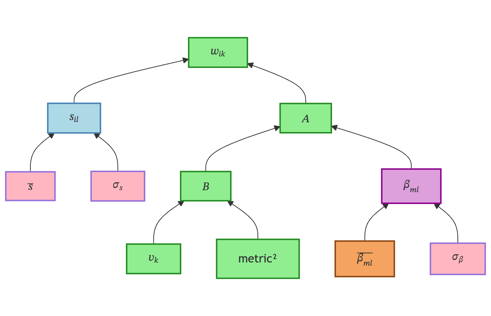
\(\gamma_k\) — Linked	Geometric trajectory: the per-feature curve. Combines `rt`, `metric`, `v0`, and `g` via parallel transport on the manifold. Code name: `model` (when no sources). Origin: `RiemanianManifoldModel.get_variables_specs()`. Definition: `LogisticModel.model_with_sources`

Spatial Variability captures how individual patients deviate from the average across features. While temporal variability shifts trajectories in time, spatial variability shifts them across the feature space — allowing, for example, one patient to have faster decline in memory but slower decline in motor skills.

Variables#
Variable & Type	Description
\(\overline{s}\) — Hyperparameter	Mean of the sources distribution. Fixed at 0 (centered prior). Code name: `sources_mean`. Origin/Definition: `TimeReparametrizedModel.get_variables_specs()`
\(\sigma_s\) — Hyperparameter	Standard deviation of the sources distribution. Fixed at 1.0 (standard normal prior). Code name: `sources_std`. Origin/Definition: `TimeReparametrizedModel.get_variables_specs()`
\(s_{il}\) — Individual latent	Source component \(l\) for patient \(i\). Sampled from \(\mathcal{N}(\overline{s},\; \sigma_s^2)\). The individual coordinates in the low-dimensional source space. Code name: `sources`. Origin/Definition: `TimeReparametrizedModel.get_variables_specs()`
\(\overline{\beta_{ml}}\) — Model parameter	Mean of the mixing coefficients. Estimated — encodes how source dimensions map to feature differences. Shape: \((d-1) \times N_s\). Code name: `betas_mean`. Origin/Definition: `TimeReparametrizedModel.get_variables_specs()`
\(\sigma_\beta\) — Hyperparameter	Standard deviation of \(\beta_{ml}\). Fixed at 0.01. Code name: `betas_std`. Origin/Definition: `TimeReparametrizedModel.get_variables_specs()`
\(\beta_{ml}\) — Population latent	Mixing coefficients. Sampled from \(\mathcal{N}(\overline{\beta_{ml}},\; \sigma_\beta^2)\). They define the mapping from source space to feature space. Code name: `betas`. Origin/Definition: `TimeReparametrizedModel.get_variables_specs()`
\(v_k\) — Linked	Velocity parameter. Input from the Geometrical Model section. Used to compute the orthonormal basis \(B\). Code name: `v0`. Origin/Definition: `RiemanianManifoldModel.get_variables_specs()`
metric² — Linked	Square of the metric tensor. Needed for the orthonormal basis computation. Code name: `metric_sqr`. Origin/Definition: `RiemanianManifoldModel.get_variables_specs()`
\(B\) — Linked	Orthonormal basis of the tangent space (perpendicular to \(v_0\)), computed from `v0` and `metric_sqr` via `OrthoBasis`. Code name: `orthonormal_basis`. Origin/Definition: `RiemanianManifoldModel.get_variables_specs()`
\(A\) — Linked	Mixing matrix: \(A = (B \cdot \beta)^T\). Maps from the source space (\(N_s\) dimensions) to the full feature space (\(d\) dimensions). Code name: `mixing_matrix`. Origin/Definition: `TimeReparametrizedModel.get_variables_specs()`
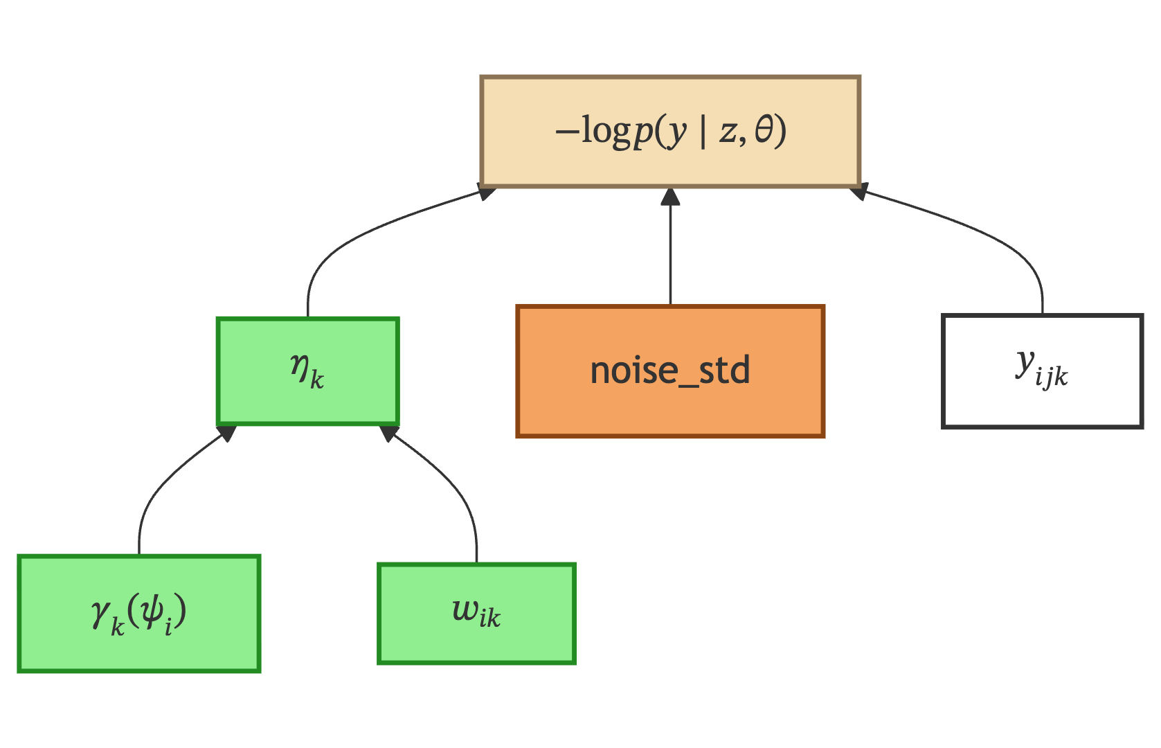
\(w_{ik}\) — Linked	Space shift for patient \(i\), feature \(k\): \(w_i = s_i \cdot A\). The individual deviation applied to each feature’s trajectory. Code name: `space_shifts`. Origin/Definition: `TimeReparametrizedModel.get_variables_specs()`

Negative Log-Likelihood is where all three branches converge. The model prediction \(\eta_k\) for each feature is compared against the observed data \(y_{ijk}\) under a noise model parameterized by the noise standard deviation.

Variables#
Variable & Type	Description
\(\gamma_k\) — Linked	Geometric trajectory from the Geometrical Model section. Code name: `model`. Origin: `RiemanianManifoldModel.get_variables_specs()`. Definition: `LogisticModel.model_with_sources`
\(w_{ik}\) — Linked	Space shift from the Spatial Variability section. Code name: `space_shifts`. Origin/Definition: `TimeReparametrizedModel.get_variables_specs()`
\(\eta_k\) — Linked	Final model prediction for patient \(i\), feature \(k\). Combines the geometric trajectory with the spatial shift: computed by `model_with_sources(rt, space_shifts, metric, v0, g)`. Code name: `model` (with sources). Origin: `RiemanianManifoldModel.get_variables_specs()`. Definition: `LogisticModel.model_with_sources`
\(y_{ijk}\) — Input data	Observed measurement. Retrieved from the `Dataset` via the observation model’s getter. Code name: `y`. Origin/Definition: `ObservationModel.get_variables_specs()`
noise_std — Model parameter	Noise standard deviation. Estimated — controls how much measurement noise is expected. Code name: `noise_std`. Origin: `FullGaussianObservationModel` (factory method). Definition: `GaussianObservationModel` (standard deviation)
\(-\log p(y \mid z, \theta)\) — Observational Model	Negative log-likelihood: computed in two stages — `nll_attach_ind` (per-individual NLL via `SumDim` over features/timepoints) then `nll_attach` (total NLL via `SumDim` over individuals). Under Gaussian noise: \(\sum_{i,j,k} \frac{(y_{ijk} - \eta_{ijk})^2}{2 \cdot \text{noise\_std}_k^2} + \text{const}\). Code name: `nll_attach`. Origin/Definition: `ObservationModel.get_variables_specs()`

Propagation example#

When the MCMC algorithm proposes a new value for \(\tau_i\):

\(\psi_i(t_{ij})\) must be recomputed (depends on \(\tau_i\))
\(\gamma_k(\psi_i(t_{ij}))\) must be recomputed (depends on \(\psi_i\))
\(\eta_k\) must be recomputed (depends on \(\gamma_k\))
The likelihood must be recomputed (depends on \(\eta_k\))
But \(g_k\), \(v_k\), \(w_{ik}\) remain unchanged — they are on different branches

The DAG encodes exactly this: sorted_children["tau"] returns the transitive closure of all downstream nodes, and the State invalidates their cached values.

How `VariablesDAG` is built#

Each model class in the inheritance chain contributes its own variables via get_variables_specs(). These contributions are accumulated using super() — each class calls super().get_variables_specs() first, then adds its own variables on top:

Class	Contributes (mathematical notation → code name)
`McmcSaemCompatibleModel`	\(t_{ij}\) (`t`), \(y_{ijk}\) (`y`), \(-\log p(...)\) (`nll_attach`)
`TimeReparametrizedModel`	\(\tau_i\), \(\xi_i\), \(\alpha_i\) (`alpha`), \(\psi_i\) (`rt`), and if multivariate: \(s_{il}\) (`sources`), \(\beta_{ml}\) (`betas`), \(w_{ik}\) (`space_shifts`), \(A\) (`mixing_matrix`)
`RiemanianManifoldModel`	\(\log(v_k)\) (`log_v0`), \(v_k\) (`v0`), metric, \(B\) (`orthonormal_basis`), \(\eta_k\) (`model`)
`LogisticModel`	\(\log(g_k)\) (`log_g`), \(g_k\) (`g`), logistic-specific metric formula

Once all specs are collected into a single dictionary, VariablesDAG.from_dict(specs) analyzes the function signatures of LinkedVariable callables to infer edges automatically. For example, LinkedVariable(Exp("log_g")) tells the DAG: “I depend on log_g”.

Relation to `State`#

The VariablesDAG is a static blueprint: it describes what variables exist and how they relate. It does not hold values.

The State object holds the runtime values for each variable. It keeps a reference to the DAG so it can propagate updates correctly. When you write state["tau"] = new_value, the State uses the DAG’s sorted_children["tau"] to invalidate all downstream caches (rt, model, nll_attach).

See StatefulModel for how the State is created and managed.